Time Series Decomposition – Algo Swing Trading

• It is the process of breaking down the series into multiple components
• This process gives us better visibility in terms of modeling complexity and which approach to follow in order to capture or model each component correctly

Lets assume a time-series with a clear trend, can be increasing on decreasing.

One of the option that we have is to remove/extract the trend component from the times series before modeling the remaining series. This will make the series stationary, and then we can add it back after the rest of the components have been used

Otherwise, we can provide enough data to the algorithm to model the trend itself

There are 2 components types in Time-Series:

• Systematic: This can be characterized by consistency which can be described and modeled

• Non-Systematic

The Following are the Systematic Components:

• Level – it the Mean Value in the series
• Trend – the change in the value between consecutive time points at any given point of time/moment. It can be associated with slop, increasing/decreasing, of the series
• Seasonality – it the deviation from the mean caused by repeating short-term cycles, with fixed and known periods

The Following are hte Non-Systematic Component:

• Noise – its the random variation in the series. This consists of all the fluctuation that are observed after removing other components (level, trend and seasonality) from the time series

Time Series Decomposition is carried out using 2 types of models:

• Additive Model
• Multiplicative Model

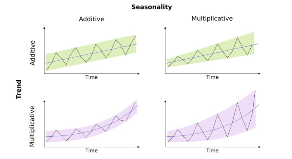
Additive Model Characteristics

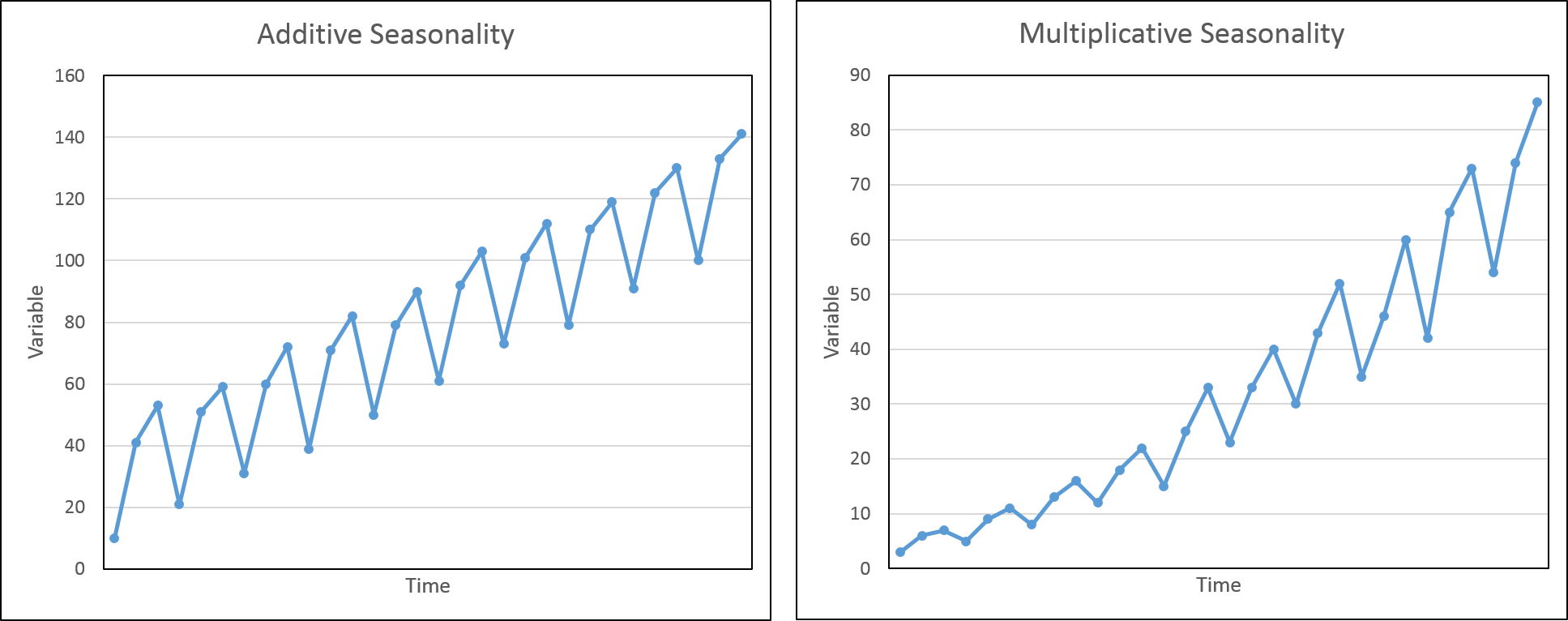
Multiplicative Model Characteristics:

• Model form y(t) = level * trend * seasonality * residue (noise)
• Changes over time is not consistent in size
• Its curved and non linear trend
• Non-linear seasonality with increasing/decreasing frequency and amplitude of cycles with time

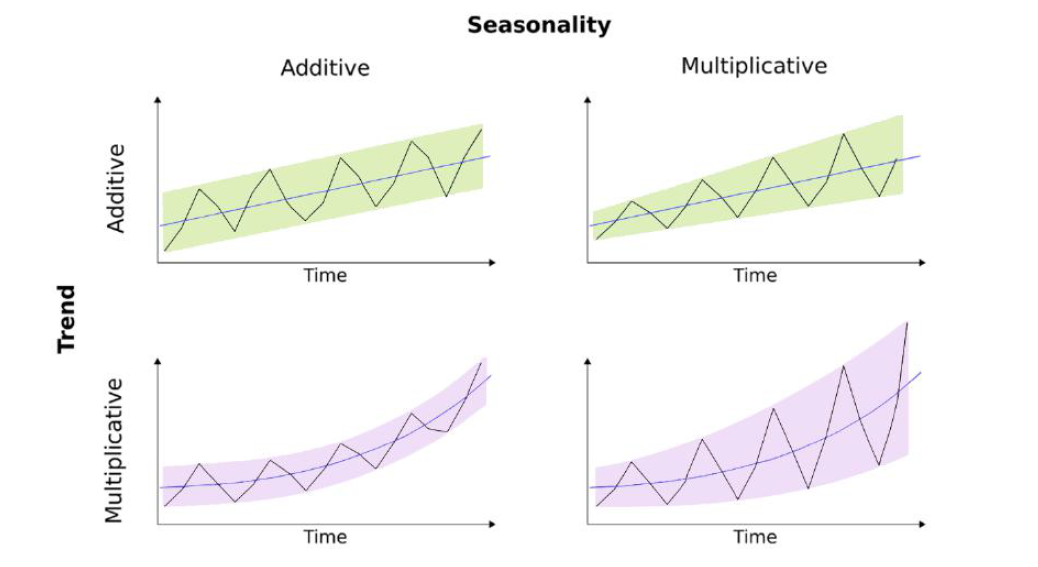
But interesting point here is, there are time-series which is the combination of additive and multiplicative characteristics, e.g series with additive trend and multiplicative seasonality

Below image can give you better understanding

Sometimes due to Model’s restriction, we can not work with the multiplicative model.

One passible solution is to transform the multiplicative model into an additive model by using logarithmic transformation

log(time * seasonality * residual) = log(time) + log (seasonality) + log(residual)

import pandas as pd
import nasdaqdatalink
import seaborn as sns
from statsmodels.tsa.seasonal import seasonal_decompose
nasdaqdatalink.ApiConfig.api_key = "xxxxx"

df = (
nasdaqdatalink.get(dataset="FRED/UNRATENSA",
start_date="2010-01-01",
end_date="2019-10-31")
.rename(columns={"Value": "unemp_rate"})
)

I did not include more recent data in this analysis, as the COVID-19 pandemic caused quite abrupt changes in
any patterns observable in the unemployment rate time series.


Add rolling mean and standard deviation:

WINDOW_SIZE = 12
df["rolling_mean"] = df["unemp_rate"].rolling(window=WINDOW_SIZE).mean()
df["rolling_std"] = df["unemp_rate"].rolling(window=WINDOW_SIZE).std()
df.plot(title="Unemployment rate")

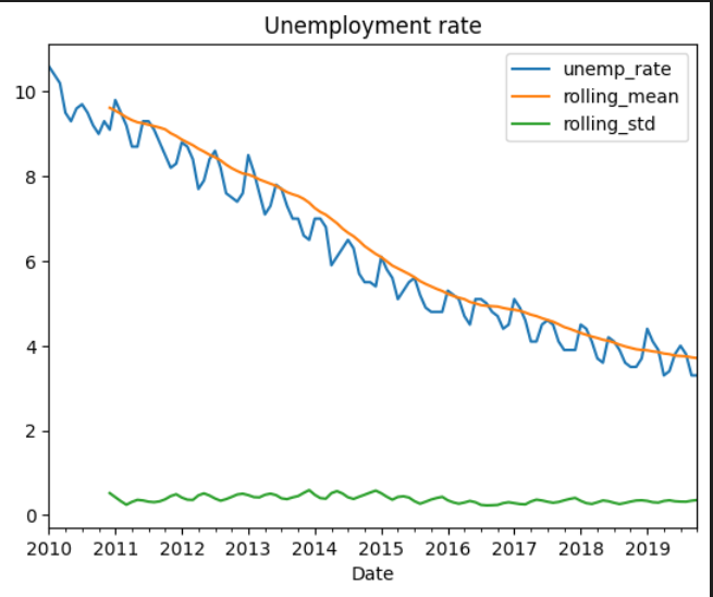
The trend and seasonal components seem to have a linear pattern. 
Therefore, we will use additive decomposition in the next step.

Carry out the seasonal decomposition using the additive model:
decomposition_results = seasonal_decompose(df["unemp_rate"],
model="additive")
(
decomposition_results
.plot()
.suptitle("Additive Decomposition")
)

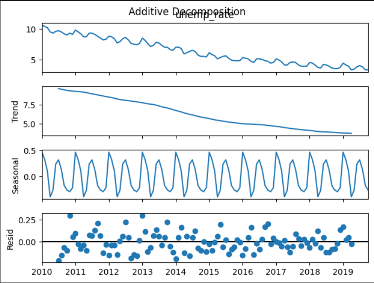
In the decomposition plot, we can see the extracted component series: trend, seasonal, and random
(residual). To evaluate the decomposition, we can look at the random component.
If there is no discernible pattern (in other words, the random component is indeed random and
behaves consistently over time), then the fit makes sense.

In this case, it looks like the variance in the residuals is slightly higher in the first half of the dataset. This can indicate that a constant seasonal
pattern is not good enough to accurately capture the seasonal component of the analyzed time series.

The seasonal decomposition we have used comes with few disadvantages:

• As the algorithm uses centered moving averages to estimate the trend, running the decomposition
  results in missing values of the trend line (and the residuals) at the very beginning and
  end of the time series.
• The seasonal pattern estimated using this approach is assumed to repeat every year. It goes
  without saying that this is a very strong assumption, especially for longer time series.
• The trend line has a tendency to over-smooth the data, which in turn results in the trend line
  not responding adequately to sharp or sudden fluctuations.
• The method is not robust to potential outliers in the data.