Introduction

• Breast cancer is one of the serious medical condition that affects millions of women worldwide.
• Recognizing and treating breast cancer is now possible but spotting it and treating it at an early stage is important.
• With Anomaly Detection we can identify tiny yet vital patterns in breast cancer that might not be visible to the naked eye.
• By increasing the accuracy of screening methods, many lives can be saved and we can help them to beat breast cancer.

Diagnosis for Breast Cancer

• Sample Collection: This process is called Biopsy. In this process, the sample of the lump is taken by using a specialized needle device, and the core of the lump is extracted from the affected area.
• Breast X-Ray: it is also called Mammogram. If there are any abnormalities found in the X-ray the doctor suggests the required treatment for further procedure.
• Ultrasound of Breast: A breast ultrasound is done to check whether the lump formed is a solid mass or a fluid-filled cyst.
• Examination of the Breast: In this, the doctor will check for lumps or any other abnormalities in both breasts.

How Machine Learning Can Help

• We can use many Machine Learning Algorithms to detect breast cancer disease which includes algorithms such as Random Forest, Logistic Regression,  SVM, Decision Trees, and Neural Networks.
• Using these algorithms, we can predict cancer at an early stage, and it will help the spreading of the disease to slow down and increases the probability of saving the life of the patient.

Objectives

• Explore the data and identify any potential anomalies.
• Create visualisations to understand the data and its abnormalities in a better way.
• Train and build a model multiple models to detect any abnormal data points.
• Will chose the best model out of 4 with multiple scoring points
• Will do Hyperparameter tuning to select the best parameter to be passed to model for better result

Common Actions on Dataset

1. Importing the Libraries
2. Loading the dataset
3. Probing Data Analysis
4. Preprocessing of the data
5. Visualising the data
6. Selecting best Algorithm
7. Hyperparameter Tuning
8. Predicting a Single Observation

Importing Libraries

import pandas as pd

Loading the Dataset / Import Data

dataset  = pd.read_csv('/content/breast_cancer_dataset
dataset

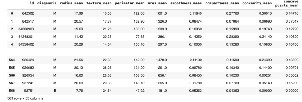
Probing Data Analysis

dataset.describe()

This will give us more information about the data like the Mean, Standard Deviation, Minimum Value of each numerical column, Mean of 25%, 50%, 75% of Data and Maximum Value of each column

dataset.shape[1]

This will give us the number of Columns in the dataset.

33

dataset.info()

This will give us the list of all Columns in the dataset with the Data Type and weather its a Nullable or Non Null Type

This is important because it will help us to categorise the column and statistical analyses can be applied to the data in order to achieve the best results. Understanding data types is also essential for successful exploratory data analysis (EDA)

len(dataset.select_dtypes(include='object').columns)

Get the number of columns that has Object Data Type

1

dataset.select_dtypes(include='float64').columns

Get all the columns which has float64 datatype

len(dataset.select_dtypes(include=['float64', 'int64']).columns)

Get the count of columns with this datatype

32

dataset.isnull().values.any()  
dataset

#checking if there any null values in the dataset

True

Checking the total Sum of Null Values

dataset.isnull().values.sum()

569

Checking which all columns have null values

dataset.columns[dataset.isnull().any()]

Number of columns having null values

len(dataset.columns[dataset.isnull().any()])

Check if we have any real number in the column

dataset['Unnamed: 32'].sum()

0.0

Drop The Columns ‘Id’ and ”Unnamed: 32” having Null Values as It is not relevant

dataset = dataset.drop(columns=['id','Unnamed: 32'])

Let’s check the dataset again

dataset.head(10)

Now we have 31 Columns left in the dataset

Confirming if we are left with any null dataset

dataset.columns.isnull().any()

False

Now Let’s work on Columns with ‘Object’ as DataType

dataset.select_dtypes(include='object').columns

Index([‘diagnosis’], dtype=’object’)
The result shows we have ‘diagnosis’ as column with object DataType

Now Lets check unique records in this column

dataset['diagnosis'].unique()

array([‘M’, ‘B’], dtype=object)
We got 2 unique items from the column

Better to Check number of unique values as well

dataset['diagnosis'].nunique()

2

Let’s Do Hot Encoding, converting categorical columns to values

dataset = pd.get_dummies(data=dataset, drop_first=True)

dataset

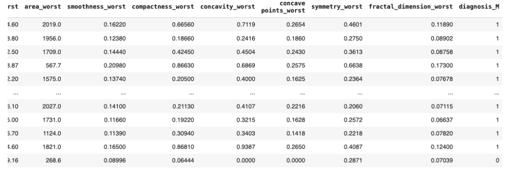
Check the result towards the end of the dataset. Here you will see ‘diagnosis_M’ column has been added in the dataset.

Hot Encoding Coverts unique values in the column to numbers and add it at the end of the dataset

Let’s Check How Many Unique Records are left in the new column

dataset['diagnosis_M'].nunique()

2

Also, let’s check if the number of rows are same in the dataset

dataset['diagnosis_M'].count()

569

Also, let’s check the DataType of newly created column

dataset['diagnosis_M'].unique()

array([1, 0], dtype=uint8)

Let’s created visualisation of the column

import seaborn as sns
import matplotlib.pyplot as plt
import numpy as np

sns.countplot(x=dataset['diagnosis_M'], label='Count')
plt.show()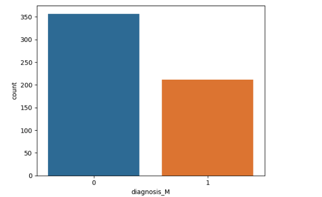

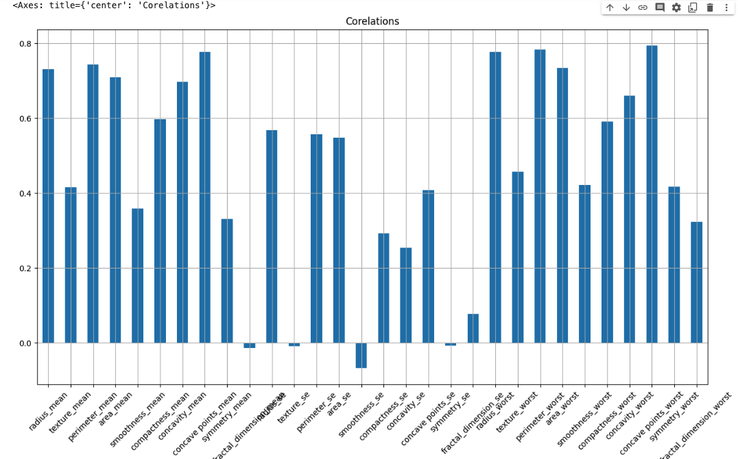
Let’s check the correlation between Features/independent Dataset with the Dependent dataset

dataset_2 = dataset.drop(columns='diagnosis_M')

dataset_2.corrwith(dataset['diagnosis_M']).plot.bar(
    grid=True, figsize=(15,8), rot=45, title='Corelations'
)

correlation matrix

corr = dataset.corr()
corr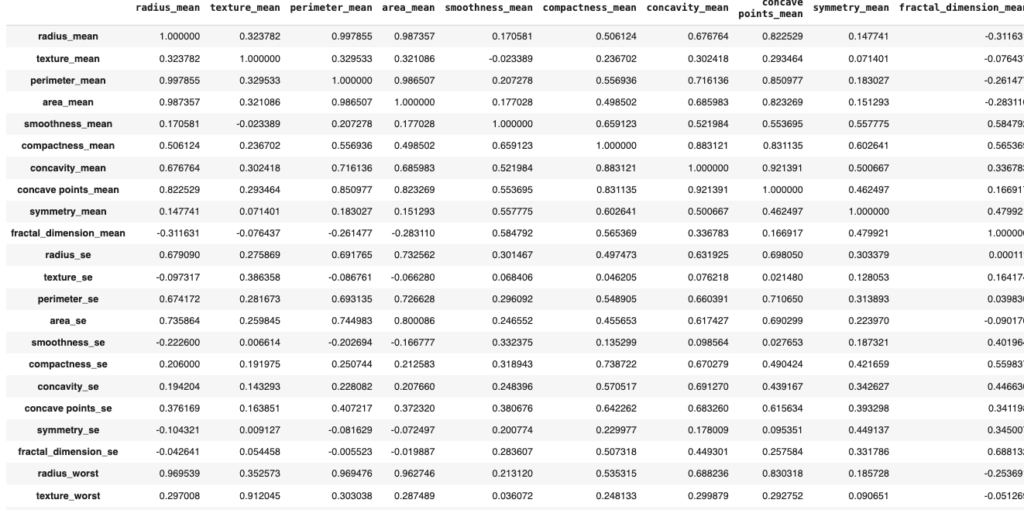

Let’s Create the heatmap of correlation matrix

plt.figure(figsize=(20, 10))
sns.heatmap(corr, annot=True)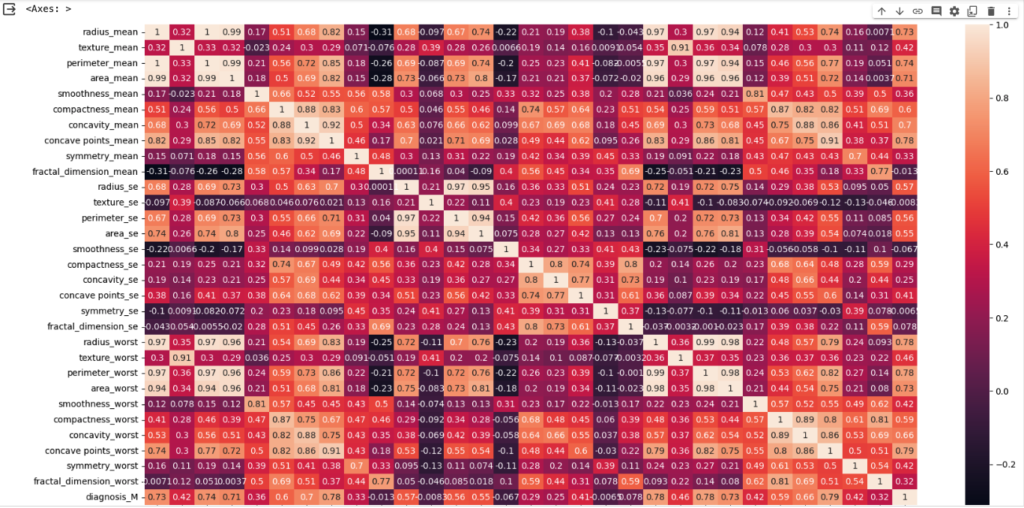

Let’s split dataset for Test and Train

First independent variable

X = dataset.iloc[:, 1:-1].values

Target/dependent variable

y = dataset.iloc[:, -1]

Let’s use class “train_test_split” from sklearn.model_selection to split the data into Test and Train Datasets

from sklearn.model_selection import train_test_split

In splitting data into Test and train dataset, we will use 20% of data and just to make sure we get same result for prediction, I will use random_state=0

X_train, X_test, y_train, y_test = train_test_split(X, y, test_size=0.2, random_state=0)

X_train.shape

(455, 29)

y_train.shape

(455,)

y_test.shape

(114,)

X_test.shape

(114, 29)

Now let’s Standardize features by removing the mean and scaling to unit variance with the help of StandardScaler

from sklearn.preprocessing import StandardScaler

Let’s create new instance of the class

scaler = StandardScaler()

For Train set we need to consider mean and std for training set

X_train = scaler.fit_transform(X_train)

To avoid over fitting we are not considering mean and std for Test Set

X_test = scaler.transform(X_test)

Feature scaling is done so that all the variables are on same scale

X_train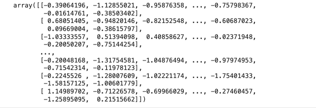

Data Preprocessing is complete here

Let’s Start Building Logistic Regression Model

Before writing code it is important to understand why we are build the model with Logistic Regression.

Logistic regression as a powerful classification algorithm using a Scikit-Learn dataset.

Logistic regression provides a simple yet effective approach for binary classification tasks, offering an interpretable and accurate model.

By leveraging the Scikit-Learn library and utilizing appropriate datasets, we can implement logistic regression with ease.

from sklearn.linear_model import LogisticRegression

logisticReg = LogisticRegression(random_state=0)

logisticReg.fit(X_train, y_train)

y_pred = logisticReg.predict(X_test)

from sklearn.metrics import accuracy_score, confusion_matrix, f1_score, precision_score, recall_score

acc_score_logisticReg = accuracy_score(y_test, y_pred)
f1_score_logisticReg = f1_score(y_test, y_pred)
pre_score_logisticReg = precision_score(y_test, y_pred)
rec_score_logisticReg = recall_score(y_test, y_pred)

result_logisticReg = pd.DataFrame(
    [['Logistic Regression', acc_score_logisticReg, f1_score_logisticReg, pre_score_logisticReg, rec_score_logisticReg]],
    columns = ['Model', 'Accuracy Score', 'F1 Score', 'Precision Score', 'Recall Score']
)

result_logisticReg

Cross Validation for Logistic Regression

conf_mat_logReg = confusion_matrix(y_test, y_pred)
conf_mat_logReg

Let’s Evaluate the Performance of Logistic Regression

from sklearn.model_selection import cross_val_score

We will take random input from X_train and y_train, and will use 10 difference accuracies based on x train and y train

print("Accuracy is {:.2f} % ".format(accu_LogReg.mean()*100))
print("Standard Deviation is {:.2f} % ".format(accu_LogReg.std()*100))

Final Result

result_logisticReg = pd.DataFrame(
    [['Logistic Regression', acc_score_logisticReg, f1_score_logisticReg, pre_score_logisticReg, rec_score_logisticReg, accu_LogReg.mean()*100, accu_LogReg.std()*100 ]],
    columns = ['Model', 'Accuracy Score', 'F1 Score', 'Precision Score', 'Recall Score', 'Cross Validation Accuracy', 'Cross Validation STD']
)
result_logisticReg

Gradient Boosting Model – XGBoost

import xgboost as xgb
xGboost_model = xgb.XGBClassifier().fit(X_train, y_train)
y_pred_xg = xGboost_model.predict(X_test)

acc_score_xGboost = accuracy_score(y_test, y_pred_xg)
f1_score_xGboost = f1_score(y_test, y_pred_xg)
pre_score_xGboost = precision_score(y_test, y_pred_xg)
rec_score_xGboost = recall_score(y_test, y_pred_xg)

result_xGboost = pd.DataFrame([['XG Boost', acc_score_xGboost, f1_score_xGboost, pre_score_xGboost, rec_score_xGboost]],
    columns = ['Model', 'Accuracy Score', 'F1 Score', 'Precision Score', 'Recall Score'])
result_xGboost

Cross Validation – Gradient Boosting Model – XGBoost

from sklearn.model_selection import cross_val_score
accuracies_xg_boost = cross_val_score(estimator=xGboost_model, X=X_train, y=y_train, cv=10 )
print("Accuracy is {:.2f} % ".format(accuracies_xg_boost.mean()*100))
print("Standard Deviation is {:.2f} % ".format(accuracies_xg_boost.std()*100))

Accuracy is 96.93 %
Standard Deviation is 1.74 %

Final Result – Gradient Boosting Model – XGBoost

result_xGboost = pd.DataFrame(
    [['XG Boost', acc_score_xGboost, f1_score_xGboost, pre_score_xGboost, rec_score_xGboost, accuracies_xg_boost.mean()*100, accuracies_xg_boost.std()*100 ]],
    columns = ['Model', 'Accuracy Score', 'F1 Score', 'Precision Score', 'Recall Score', 'Cross Validation Accuracy', 'Cross Validation STD']
)
result_xGboost

result = pd.concat([result_logisticReg, result_xGboost],ignore_index=True)
result

Random Forest

from sklearn.ensemble import RandomForestClassifier
model_RanFor = RandomForestClassifier(random_state=0)
model_RanFor.fit(X_train, y_train )
y_pred_RanFor = model_RanFor.predict(X_test)

acc_score_RanFor = accuracy_score(y_test, y_pred_RanFor)
f1_score_RanFor = f1_score(y_test, y_pred_RanFor)
pre_score_RanFor = precision_score(y_test, y_pred_RanFor)
rec_score_RanFor = recall_score(y_test, y_pred_RanFor)

result_RanForm = pd.DataFrame(
    [['Random Forest', acc_score_RanFor, f1_score_RanFor, pre_score_RanFor, rec_score_RanFor]],
    columns = ['Model', 'Accuracy Score', 'F1 Score', 'Precision Score', 'Recall Score']
)
result_RanForm

keyboard_arrow_down

Cross Validation RF

from sklearn.model_selection import cross_val_score
accuracies_RandFor = cross_val_score(estimator=model_RanFor, X=X_train, y=y_train, cv=10 )
print("Accuracy is {:.2f} % ".format(accuracies_RandFor.mean()*100))
print("Standard Deviation is {:.2f} % ".format(accuracies_RandFor.std()*100))

Accuracy is 95.83 %
Standard Deviation is 3.01 %

Final Result RF

result_RanForm = pd.DataFrame(
    [['Random Forest', acc_score_RanFor, f1_score_RanFor, pre_score_RanFor, rec_score_RanFor, accuracies_RandFor.mean()*100, accuracies_RandFor.std()*100 ]],
    columns = ['Model', 'Accuracy Score', 'F1 Score', 'Precision Score', 'Recall Score', 'Cross Validation Accuracy', 'Cross Validation STD']
)
result_RanForm

result = pd.concat([result,result_RanForm], ignore_index=True)
result

Support Vector Machine (SVM)

from sklearn.svm import SVC
svm_model = SVC().fit(X_train, y_train)
y_pred_svm = svm_model.predict(X_test)

acc_score_svm = accuracy_score(y_test, y_pred_svm)
f1_score_svm = f1_score(y_test, y_pred_svm)
pre_score_svm = precision_score(y_test, y_pred_svm)
rec_score_svm = recall_score(y_test, y_pred_svm)

result_svm = pd.DataFrame([['SVM', acc_score_svm, f1_score_svm,pre_score_svm, rec_score_svm, ]],
    columns = ['Model', 'Accuracy Score', 'F1 Score', 'Precision Score', 'Recall Score']
)
result_svm

Cross Validation

accuracies_svm = cross_val_score(estimator=svm_model, X=X_train, y=y_train, cv=10 )
print("Cross Valiataion Accuracy for SVM is {:.2f} % ".format(accuracies_svm.mean()*100))
print("Cross Valiataion Standard Deviation for SVM is {:.2f} % ".format(accuracies_svm.std()*100))

Cross Valiataion Accuracy for SVM is 97.81 %
Cross Valiataion Standard Deviation for SVM is 1.39 %

Final Result SVM

result_svm = pd.DataFrame(
    [['SVM', acc_score_svm, f1_score_svm, pre_score_svm, rec_score_svm, accuracies_svm.mean()*100, accuracies_svm.std()*100 ]],
    columns = ['Model', 'Accuracy Score', 'F1 Score', 'Precision Score', 'Recall Score', 'Cross Validation Accuracy', 'Cross Validation STD']
)
result_svm

result = pd.concat([result,result_svm], ignore_index=True)

result

Choose Model For HyperParameter Tuning

Since SVM and Logistic Regression have same validation Accuracy but SVM has less STD, we will take SVM for Hypertuning

from sklearn.model_selection import RandomizedSearchCV
from scipy.stats import uniform
import random

param_dist = {
    'C': uniform(0.1, 10),
    'kernel': ['linear', 'rbf', 'poly'],
    'gamma': ['scale', 'auto'] + list(np.logspace(-3, 3, 10)),
}
param_dist

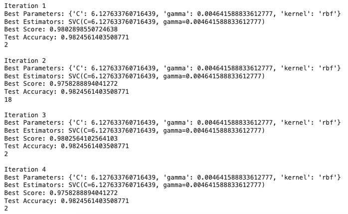
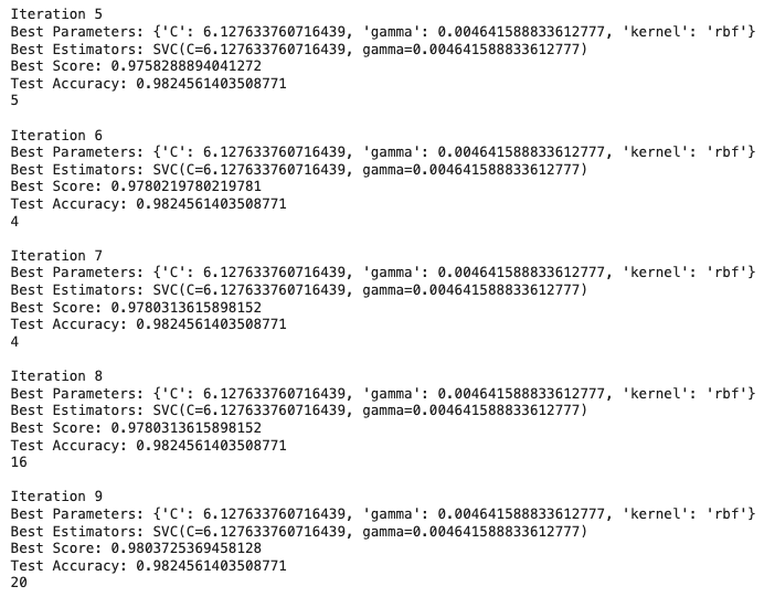
max_iterations = 10
iteration = 1

while iteration <= max_iterations:
    n_itr_ran=random.randint(0,20)
    print(n_itr_ran)
    print(f"\nIteration {iteration}")

    # Perform RandomizedSearchCV
    random_search = RandomizedSearchCV(svm_model, param_distributions=param_dist, n_iter=n_itr_ran, cv=n_itr_ran, random_state=0)
    random_search.fit(X_train, y_train)

    # Display the best parameters
    print("Best Parameters:", random_search.best_params_)
    print("Best Estimators:", random_search.best_estimator_)
    print("Best Score:", random_search.best_score_)

    # Update the SVM model with the best parameters
    best_params = random_search.best_params_
    svm_model.set_params(**best_params)

    # Train the model with the updated parameters
    svm_model.fit(X_train, y_train)

    # Evaluate the model on the test set
    accuracy = svm_model.score(X_test, y_test)
    print("Test Accuracy:", accuracy)

    # Increment the iteration counter
    iteration += 1